Building a Robot Arm That Can See

In 2021, for a robotics class at WPI, I built a robot arm that could look at a table, find colored balls, pick them up, and sort them into bins.

The project became a compact lesson in robotics: perception is not useful until it is connected to coordinates, coordinates are not useful until they are connected to motion, and motion is not useful if the hardware destroys itself on the way there.

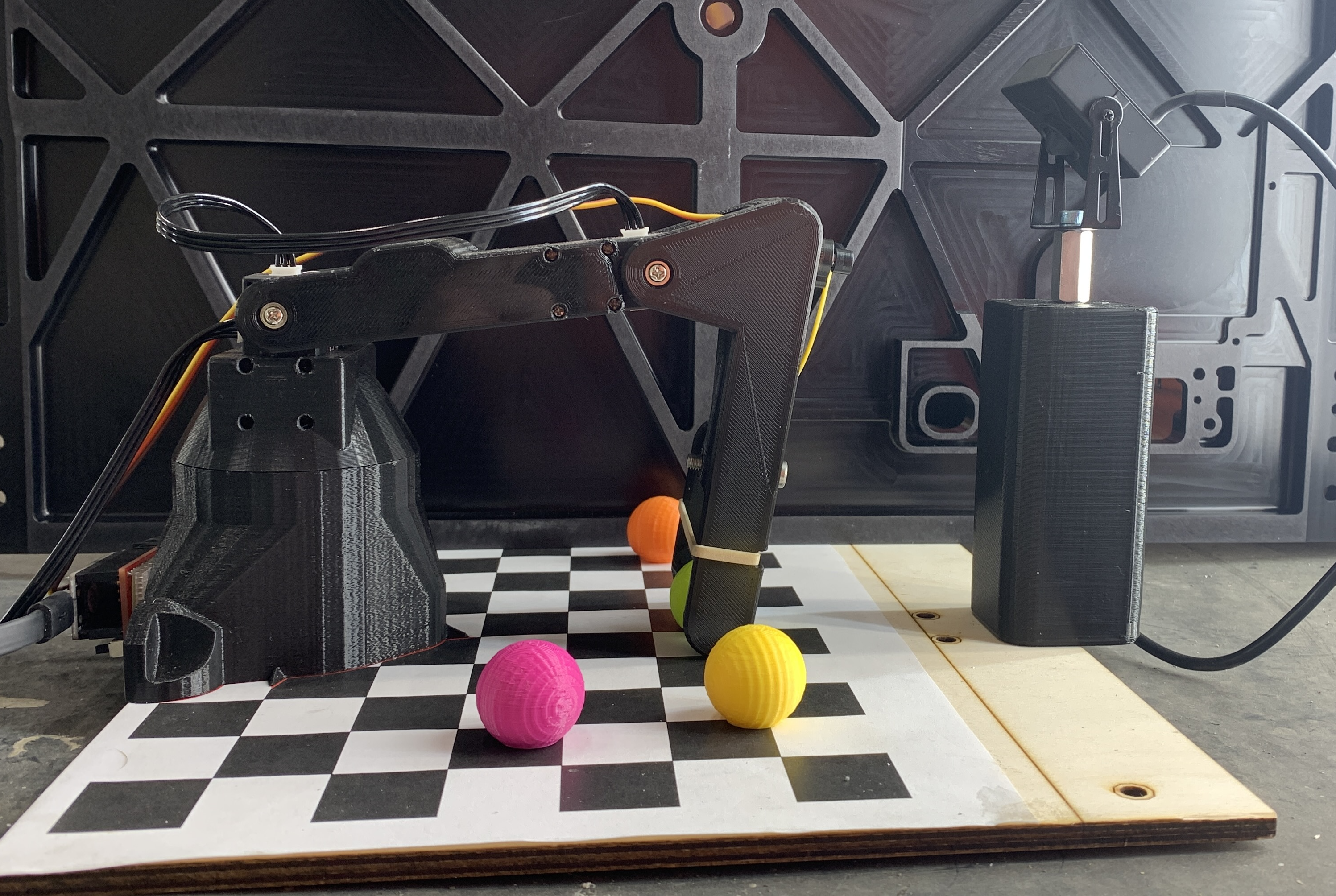
On hardware:

• The arm only had three degrees of freedom and a small gripper.
• The camera was a cheap fisheye camera.
• The 3D-printed structure flexed, the servo horns could strip if we moved too aggressively, and every small error—camera distortion, calibration, kinematics, mechanical backlash—eventually accumulated at the gripper.

The challenge: a tiny produce picker

The assignment was to sort similarly sized balls by color. We treated the balls as produce: ripe and unripe tomatoes that needed to be identified, picked, and placed into separate containers.

Our team was Nico Machado, Jeremy Trilling, and me. We called the system the Produce Picker, and built it during COVID while each of us worked remotely with our own robot, camera, computer, and lighting conditions.

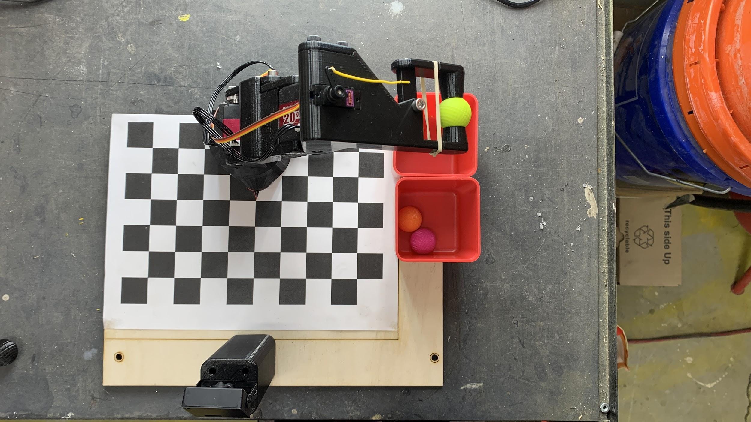
The finished loop needed to:

1. Take a picture of the checkerboard workspace.
2. Find a ball and calculate its center in image pixels.
3. Convert that pixel into a position in the checkerboard frame.
4. Transform the position into the robot's base frame.
5. Solve for the joint angles that put the gripper above the ball.
6. Move without hitting the ball or entering a singularity.
7. Close the gripper, lift the ball, and place it in the correct bin.
8. Repeat until the workspace was clear.

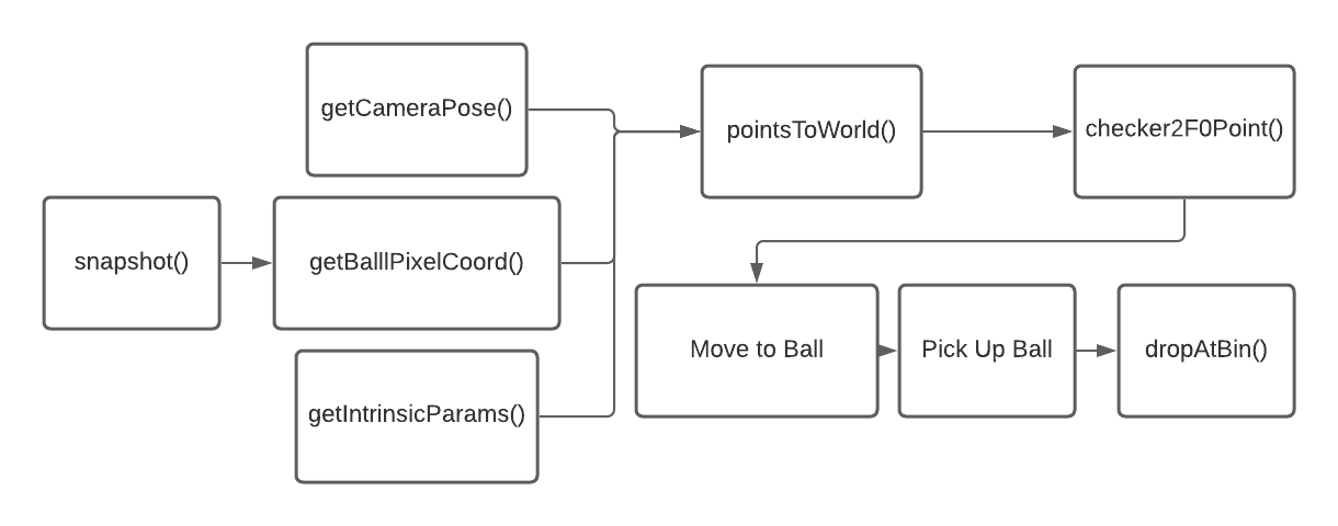
Each box in the diagram is understandable on its own. The hard part is making every box agree about where the world is.

The project was really four labs wearing a trench coat

The final system did not appear all at once, but through four iterations.

Step 1: Real time doesn't mean fast, it means consistent

We assembled the three-degree-of-freedom arm, post-processed the 3D-printed frame parts, soldered the power distribution board, assigned IDs to the smart servos, and calibrated their zero positions. We configured Linux workstations with MATLAB, then wrote the first wrapper functions for commanding and measuring the joints:

• servo_jp() sent joint positions directly.
• interpolate_jp() requested an interpolated joint move.
• measured_js() read the measured joint state.
• setpoint_js() read the current controller setpoint.
• goal_js() read the final commanded joint goal.

One of the first experiments compared an interpolated move with a direct command. The direct command reached the target quickly, but its acceleration was abrupt and the other joints showed more disturbance. Interpolation took longer and produced a gentler profile.

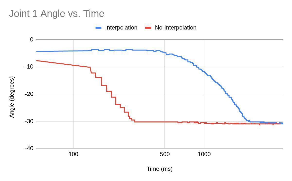
The chart also exposed a less glamorous problem: our MATLAB loop was not real-time. Samples could be separated by a millisecond or by roughly 100 milliseconds depending on CPU load and the computer running the code. "Run the loop as fast as possible" is not the same thing as "run the loop at a dependable rate." Any controller that assumes a fixed timestep needs an actual timer.

This became important later, when trajectory evaluation and velocity calculations depended on elapsed time.

Step 2: teach the robot its own geometry

Next we built a forward-kinematics model using Denavit-Hartenberg parameters. The arm had a 95 mm vertical offset from the base followed by two 100 mm links. We assigned a coordinate frame to each joint, formed the intermediate homogeneous transforms, and multiplied them to get the transform from the base to the end effector.

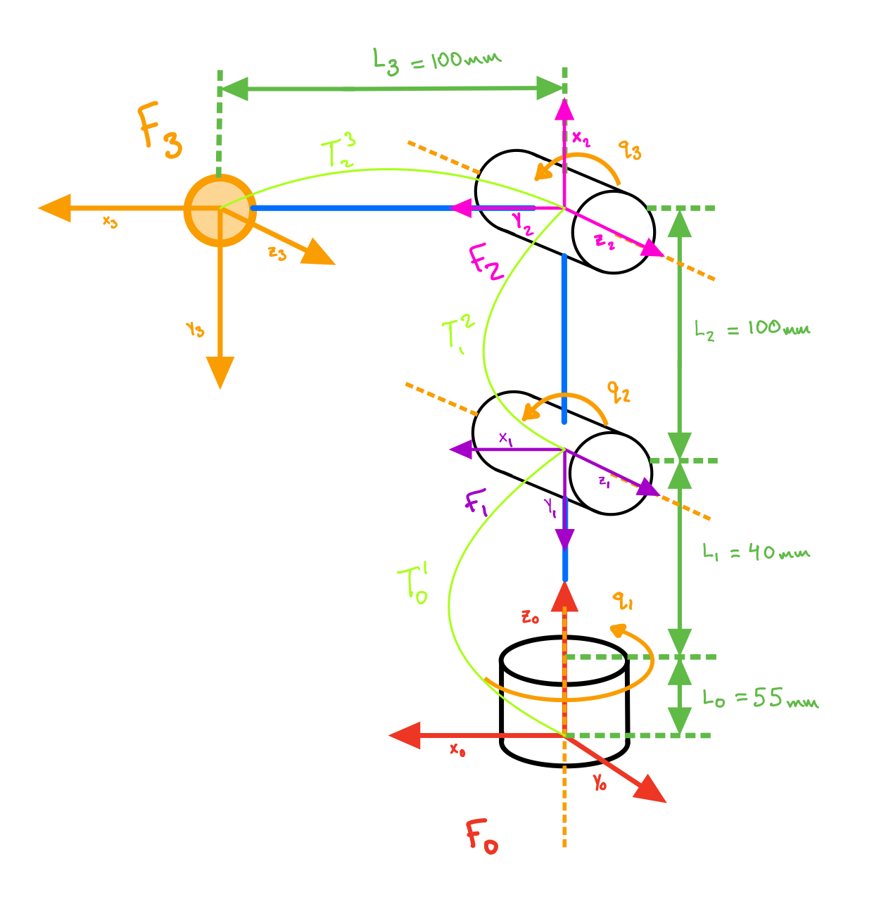
This gave us several useful functions:

• dh2mat() converted one DH row into a homogeneous transform.
• dh2fk() chained a DH table into a complete forward-kinematics result.
• fk3001() specialized the calculation for our arm.
• measured_cp(), setpoint_cp(), and goal_cp() exposed measured, setpoint, and goal positions in Cartesian space.

We created a live MATLAB stick model that followed the physical arm, commanded arbitrary points, and traced triangles in different planes. The X-Z triangle held the base joint still. The X-Y triangle required all three joints and was noticeably harder to place accurately.

When we repeatedly commanded one task-space point, the measured tip position had an RMS magnitude error of 6.5008 mm. Six and a half millimeters sounds small until the object you are trying to grab is only a few times wider than that.

We also sampled the joint limits to visualize the theoretical workspace:

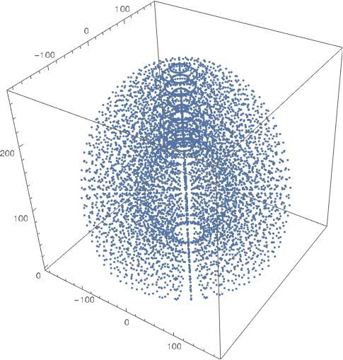
The plot is a useful reminder that "reachable" is not binary. A point can be inside the geometric workspace but near a poor configuration, outside the camera's clean field of view, or reachable only with a path that collides with the table.

Step 4: Velocity: The difference between a produce picker and fruit ninja.

Position kinematics tells you where the gripper is. Velocity kinematics tells you how joint motion becomes gripper motion.

We derived the six-row Jacobian, with the translational component on top and rotational component below. In compact form:

That let us calculate task-space velocity from joint velocity. Running it backward let us estimate joint velocities needed to follow a task-space direction.

We implemented:

• jacob3001() to evaluate the Jacobian for the current joint configuration.
• fdk3001() for forward differential kinematics.
• ik_3001_numerical() for iterative inverse kinematics.
• is_close_to_singularity() as a safety check.

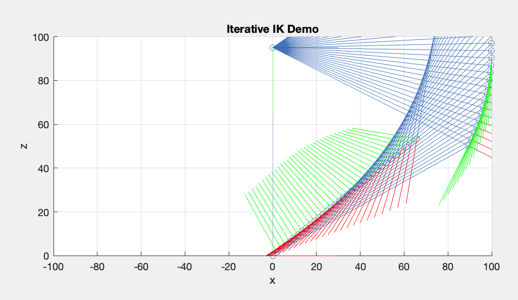
The numerical IK solver repeatedly used inverse velocity kinematics to move the model closer to a requested point. It was a useful general method, even though the final project's simple three-joint geometry also allowed us to derive a closed-form position solution.

The Jacobian introduced us to singularities: configurations where the robot loses motion authority in one direction. We watched the determinant of the translational portion. Two known singular configurations produced determinants of zero or effectively zero; a safer test configuration produced a determinant of 500,000.

Without safety code, the physical consequence was more memorable than the matrix. Our arm started wildly flailing in a circle.

Less produce picker and more fruit ninja.

Step 5: Make it See

The final project combined all of the earlier work with camera calibration, color segmentation, coordinate transforms, a state machine, and grasp planning.

In other words, we finally made every previous source of error meet in the same place.

Solving the arm backward

Forward kinematics answers:

If the joints are at these angles, where is the gripper?

Picking requires the inverse question:

If the ball is here, what should the joint angles be?

For the final controller, the first joint angle came from the target's direction in the X-Y plane:

After that rotation, the remaining two joints reduced to a planar two-link geometry problem.

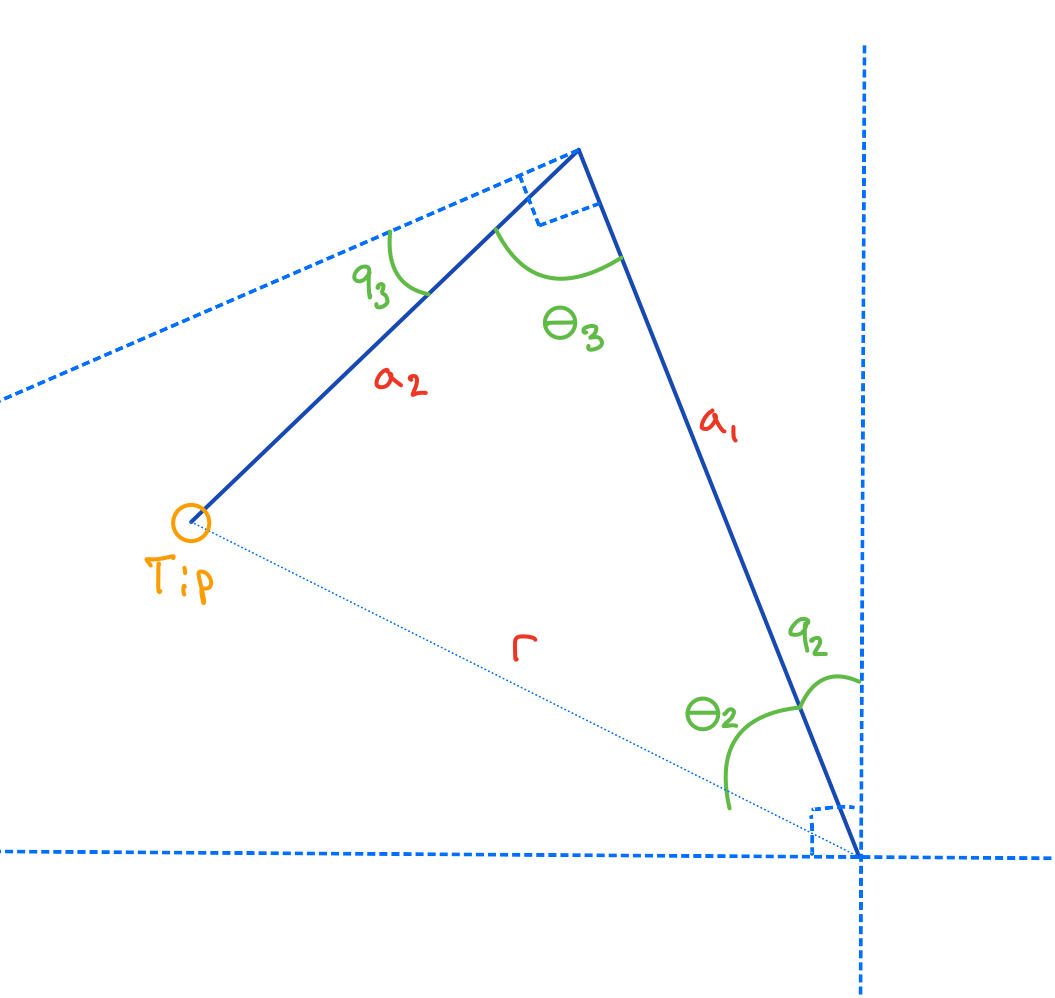
With the 95 mm base height removed from the target Z coordinate, we calculated the radial distance to the target, used the law of cosines for the shoulder and elbow solutions, then chose a joint configuration the physical arm could actually use.

There can be more than one mathematical answer. "Elbow up" and "elbow down" may both reach the same point, but only one may stay above the table or within the joint limits. The inverse-kinematics function therefore needed to return more than correct angles; it needed to return a usable posture.

Teaching a camera to speak millimeters

A camera does not naturally return millimeters. It returns pixels.

We calibrated the fisheye lens using twenty images of a 9-by-13 checkerboard taken from different positions and angles. MATLAB estimated the camera intrinsics, including nonlinear lens distortion, and calculated the reprojection error for every calibration image.

Six of the twenty images were rejected for excessive error. The fourteen retained images had an overall mean reprojection error of about 0.83 pixels.

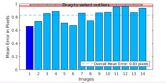
The team also plotted each checkerboard pose in 3D. That showed whether the calibration dataset surrounded the workspace or repeated too many similar viewpoints. Calibration is not just collecting more pictures; it is collecting pictures that constrain the model from meaningfully different perspectives.

Once the camera was calibrated, we estimated its pose relative to the checkerboard. A detected pixel could then be projected onto the board plane and transformed into the robot's base frame.

Conceptually, the coordinate chain looked like this:

The annoying detail was that a ball's visible center is not on the checkerboard plane. It sits above the board. If we projected that center as if it were flat on the board, perspective shifted the estimated position away from the camera.

We tried tolerating the error because the gripper had a wide mouth. That worked near the center of the workspace and failed near the edges. We then derived a geometric correction using the camera position, the board-projected point, and similar triangles to pull the estimate toward the ball's real location.

Finding ripe and unripe "produce"

We used HSV color rather than raw RGB values. Hue describes the color family, while saturation and value can absorb more of the variation caused by shadows and illumination. That mattered because three people were testing the same code with three cameras under three different lighting setups.

Our original design divided the hue wheel into ripe and unripe regions. In the final code, MATLAB's Color Thresholder helped us tune masks from real test images.

The detection pipeline stayed deliberately simple:

1. Take a camera snapshot.
2. Convert the image from RGB to HSV.
3. Threshold the selected color into a binary mask.
4. Combine it with a region-of-interest mask for the checkerboard.
5. Run regionprops() on connected regions.
6. Reject noise using area and circularity.
7. Return the centroid of the next valid ball.

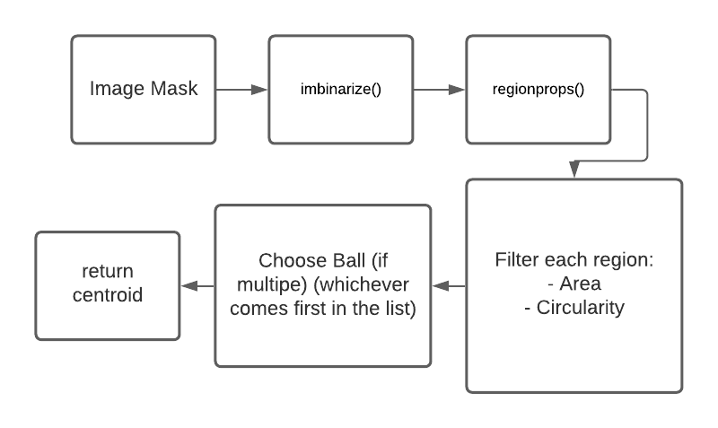
The region-of-interest mask was especially valuable. Instead of asking the detector to understand the entire room, we told it that nothing outside the checkerboard could be a valid target. Removing irrelevant reality is often cheaper than modeling it.

There was one funny limitation: the black balls looked too much like the black squares of the checkerboard. The camera was being asked to distinguish two objects whose most important visual feature was intentionally identical.

Sometimes the best vision algorithm is changing the scene. Sometimes it is admitting that the scene is ambiguous and not picking the black ball.

Why we used quintic trajectories

Early in the course we let the servo firmware interpolate joint commands. We also experimented with cubic and velocity-based motion. For the final project, we generated a quintic polynomial independently for each task-space axis.

A fifth-order polynomial provides six coefficients, enough to constrain position, velocity, and acceleration at both ends of a move. We could begin and end with zero velocity and zero acceleration, then evaluate the polynomial at the current elapsed time to produce a smooth task-space setpoint.

At each update:

1. Evaluate the X, Y, and Z quintics.
2. Solve inverse kinematics for the resulting point.
3. Send the joint-angle setpoint to the servo controller.
4. Repeat until the trajectory time expires.

This was not just aesthetic smoothness. At full servo speed, the arm generated enough torque to strip the splines in the servo horns. We reduced maximum acceleration because the software's fastest possible motion was outside the mechanical system's comfort zone.

A more sophisticated system could model forces with a Lagrangian and use torque propagation or closed-loop torque control. For this arm, acceleration-limited quintic motion was the practical solution.

Step 5: Putting it all together

My direct contributions included parts of the computer-vision pipeline, the inverse-kinematics functions, system architecture, and experiments comparing trajectory error between motion strategies. The project was a team effort with Nico Machado and Jeremy Trilling.

What I took away

This was not the most advanced robot I worked on at WPI, but it compressed a surprising amount of robotics into one tabletop system.

My biggest takeaway:

• The physical world demands compromises.

The camera can be off by less than a pixel. The kinematics can be off by a few millimeters. The servo can have a little backlash. The gripper can flex. The ball can roll. No single error looks fatal, but the robot experiences their sum.

Robotics is the work of closing those gaps until the machine finally does the thing you meant.